3. Project Management: Let’s Get Organized

Know where you are…

Learning objectives

• Understand motivation for project based workflows
• Know how to organize code, data, and results
• Know the basics of file paths and directory structures
• Be able to create and use an RStudio project

Where Am I?

Figure 1: A disorganized system for finding things

Any time you are working on your computer, you must navigate amidst a forest of files and folders.

One of the most common issues we deal with in R programming is to tell your computer where a file or folder is located.

Thus, one of the most useful habits you can form (whether using R or not), is to intentionally keep a clear structure and use that same structure across all of your projects. This becomes especially important when using computer programming languages like in your work. You will need to tell R, very specifically, where you are and where your files are located in the forest of your computer.

Where you are is typically referred to as the working directory. The working directory is a folder. In , think of this as your homebase, and everything is relative to this folder on your computer.

Use Project Workflows

One of the great advantages of using tools like RStudio is they make it easy to use an organized “project” workflow. What do we mean by “using projects”? Projects refer to a general pattern or structure used for each work project or analysis. This approach is not specific to R. Any practiced data scientist will use a folder structure and organization scheme, no matter what programming language they use.

The general idea is to always use the same structure and naming schemes across every project. Do this every single time with every single project you make, in order to make it a habit. This will save you time and brainpower! Imagine quickly moving between tasks or projects with minimal time spent “trying to find where things are and getting oriented”. You’ll always know where things should be!

Basic Folders for Every Project

At a minimum, it’s useful to have separate directories (folders) for each of the following:

• data: Ideally keep data in a .csv format, because these simple and universal data. You may have other specialized formats as well. This is generally where original, raw data lives.
• data_output: This is where you save any data or analysis outputs. Any time you clean, tidy, summarize, or otherwise manipulate the data and save it out, it should end up somewhere clearly different than the raw data location.
• scripts: In the world, “scripts” are generally .R files. However, you may have .do files if wokring with Stata, .py files for Python, and so on. Using a sequential numbering file naming scheme can be useful. Remember to pad with a zero to make file sorting/ordering easy (e.g., 00_script_a.R, 01_script_b.py, etc).
• results: These may include model results, data analysis, slides, and so on. Some like to keep figures in this folder and others prefer a specific figures folder.
• documents: This is a place you can keep documents, papers, pdfs, etc. These may include files with .docx, .Rmd (for RMarkdown), .pdf or even .html extensions.

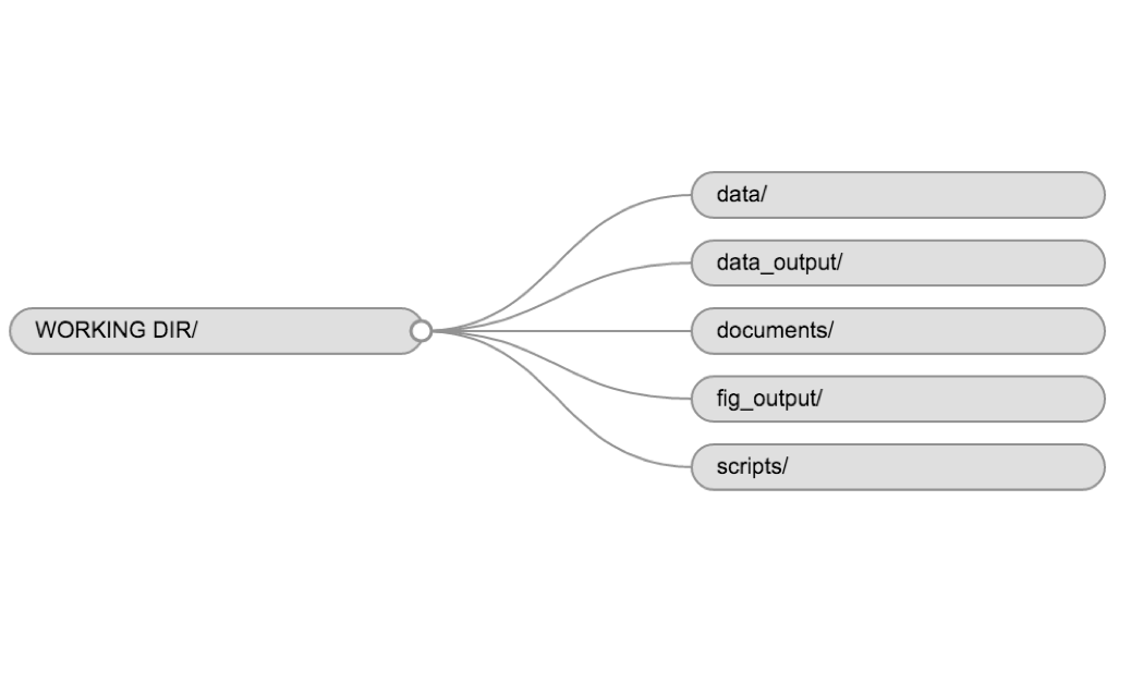
Figure 2: An example project folder structure

RStudio Projects

Within the R environment, something that makes project management and organization much easier is the use of RStudio Projects (.Rproj file). RStudio makes the use of Projects straightforward. One of the nicest parts of using RStudio Projects is that they automatically set the working directory to the folder containing a specified .RProj file. You can make any existing folder an RProject folder, or make a new one. RStudio projects are a great way to quickly and easily organize your workflows; each project can be a specific task, or a larger set of objectives you need to complete. With RStudio Projects, it’s easy to switch between projects, or work on different projects simultaneously without much mental overload, especially if you use the same project folder structure across each project!

Avoid using setwd()! More reasons and rationale linked here.

Setting up an .Rproj

Let’s create an RStudio Project as part of this course that you can use throughout each module. We highly recommend that no matter what you are working on in R, that you try to do it within the structure of an RStudio Project!

1. Open RStudio and navigate to the upper right-hand side where it says “Project: (None)”. If we click on this button, we should see some options. Select New Project.
2. We can use either a New Directory, or setup a project in an Existing Directory. Both give similar options.
3. Select “New Project”

Figure 3: RStudio Project setup

4. Make a new sub-directory folder (if you don’t have it) under your Documents folder called: Rprojects

It’s a good idea to keep all your R projects in one place. You can decide if this should be in your ~/Documents folder, or somewhere else (associated with a version control or cloud service like Dropbox/Box/etc).

5. Finally, we can name our new project (remember no spaces in our folder/file names!): intro_r4wrds

Figure 4: Make a new project named intro_r4wrds

Make Folders & Add Data

Great! Now we can create a folder structure in our project as discussed in the Basic Folders for Every Project section above. More importantly, we can also put all our course data into the data folder in your RStudio project.

We can’t drag and drop files from an Explorer or Finder window directly into RStudio. We can only go from Explorer to Explorer. In the Files tab, click on More with the little , and then select “Show Folder in New Window”.

Let’s go ahead and make the following folders (HINT: you can use the “New Folder” button in RStudio, or use the code below!)

• data
• data_output
• figures
• scripts

Then in your Console tab, you can enter this code to download the data directly into your project!

dir.create("data") # warning is ok if already exists!

# downloads the file (data.zip) to your data directory
download.file("https://github.com/r4wrds/r4wrds-data-intro/raw/main/data.zip", destfile = "data/data.zip")

# unzip the data we need for the course:
unzip(zipfile = "data/data.zip")

File Paths

In R, file paths are always wrapped in quotes. There are 2 basic kinds of file paths:

• Absolute: Absolute paths list out the full file path, usually starting with your username, which you can also refer to using the shortcut ~. So instead of C:/MyName/Documents or /Users/MyName/Documents, you can type ~/Documents. But generally, the only place an absolute path will work is your computer! It will break on anyone else computer, or anytime you move or rename something!

• Relative: Relative paths are relative to your working directory. So if R thinks we’re in that ~/MyName/Documents/Projects/2020 folder, and we want to access a file in a folder inside it called data, we can type data/my_file instead of ~MyName/Documents/Projects/2020/data.

The good news is if you setup an RStudio project as shown above, you can use relative filepaths with ease!

The Working Directory

Our working directory should be the root place where our project lives (as shown above). You can always check what R thinks is the working directory with getwd(), and you should see the folder where your .Rproj file lives! Importantly, everything you do should be relative to that working directory.

That means we really don’t want to use things like setwd() (set working directory) to locate a file or folder on our computer, or use a hard path (i.e., a full path like C:/MyUserName/My_Documents/A_Folder_You_May_Have/But_This_One_You_Definitely_Dont/). That’s because this will pretty much never work on anyone’s computer other than your own, and sometimes it may not even work on your own computer if you change a file name or folder! How can we make things reproducible for others, and for our future self? We advise using the {here} package.

Using the {here} package

Good news! There’s a package designed to make project-based workflows work so that code is portable between machines (i.e., you can share your project with a collaborator and they don’t need to fiddle with working directories and file paths). The {here} package makes it easy to create a path relative to the top-level directory (the place where your current project is) with a single function: here(). In addition, we can use here() to build a relative path to a file for saving or loading. Let’s say we’re working in our MyName/Documents/Projects/2020 folder.

library(here)

# identify your working directory.
here()

# will be something like this:
#> [1] /Users/MyName/Documents/Projects/MyProject

# read a file from our data folder! `data/nwis_sites_american_river.csv`
read.csv(here("data", "nwis_sites_american_river.csv"))

Figure 5: Illustration by @allison_horst.

Using the {here} package means we can share our project with other folks and it will work, and if something changes around inside the project, it will remain functional and accessible.

In practice however, if we always work from within an RProject, we can simply use relative paths without the here() syntax – that syntax just makes it very explicit what we’re doing.

Best Practices: Project Organization/Workflow Tips

Although there is no “best” way to lay out a project, there are some general principles to adhere to that will make project management easier. Here’s some sage advice from Jenny Bryan and Jim Hester from What They Forgot to Teach you About R (worth checking out!):

• File system discipline: put all the files related to a single project in a designated folder.
• This applies to data, code, figures, notes, etc.
• Depending on project complexity, you might enforce further organization into subfolders.
• Use a standard naming convention for files & folders (no spaces!).
• Don’t use absolute paths!
• File path discipline: all paths are relative and, by default, relative to the project’s (your working directory) folder.

Always start R as a blank slate

When you quit R, do not save the workspace to an .Rdata file. When you launch, do not reload the workspace from an .Rdata file.

In fact, we should all make our default setting a blank slate. We should only be loading and working on data and code that we knowingly and willingly open or import into R.

In RStudio, set this via Tools > Global Options

(ref:workspaceDef) Change defaults to never save your workspace to .RData! (Credit to Jenny Bryan and Jim Hester at rstats.wtf)

Figure 6: (ref:workspaceDef)

Safe File Naming

This is really important and will make life easier for everyone in the long run. Jenny Bryan has the best set of slides on this, so take a few minutes and go read them. Then be the change!

Slides You Need to Read

TL&DR (Too long, didn’t read)

• File names should be machine readable (i.e., no spaces)
• Human readable (m_import_clean_data.R)
• Makes default ordering easy (i.e., dates are always YYYY-MM-DD)

Treat raw data as Read Only

This is probably the most important tip for making a project reproducible and hassle free. Raw data should never be edited, because you don’t want to permanently change your starting point in an analysis, and you want to have a record of any changes you make to data. Therefore, treat your raw data as “read only”, perhaps even making a raw_data directory that is never modified. If you do some data cleaning or modification, save the modified file separate from the raw data, and ideally keep all the modifying actions in a script so that you can review and revise them as needed in the future.

Treat generated output as disposable

Anything generated by your scripts should be treated as disposable: it should all be able to be regenerated with code. Don’t get attached to anything other than your raw data, and your code! There are lots of different ways to manage this output, and what’s best may depend on the particular kind of project.

Summary

There are many ways to use project-based workflows in R. Importantly, we advise that you find a strategy that works for the majority of the work you do, and then be consistent about organizing things the same way (from folder structure to file naming). This will help folks you work with, it will help you (including your future self), and you spend less time figuring out where you are (and where the pieces you need to do work with are) and more time doing the work you need to do!

Lesson adapted from R-DAVIS, Jenny Bryan and Jim Hester’s What they forgot to teach you about R, and the Data Carpentry: R for data analysis and visualization of Ecological Data lessons.

Previous module:
2. Getting started Next module:
4. Import/export data