13. Intro to Rmarkdown

Save time and have fun with reproducible documents + code!

Learning Rmarkdown

• Learn the main components of an Rmarkdown (.Rmd) document
• Understand how to create a new Rmd and add text and images
• Learn how to stitch (or knit) a document together and share it

Rmarkdown: Knitting Things Together

This entire course website is built using Rmarkdown files. Dissertations, papers, reports, and interactive documents are all very possible using Rmarkdown. While it would be impossible to show you how to do all of these things, the good news is while Rmarkdown is highly customizable, there are only a few key components to learn. We’ll go over some of the main pieces, demonstrate some fun tricks that are made easy using Rmarkdown, and provide a bunch of great resources to help you learn more!

Check out the RMarkdown Gallery for examples and inspiration.

(ref:AHrmdplot) Illustration by @allison_horst

Figure 1: (ref:AHrmdplot)

Reproducible

Depending on the tasks you are faced with, analysis is rarely something that happens a single time. We are constantly faced with tasks (sometimes small, sometimes large) that have repetitive information, or repetitive steps to complete. Making this process more reproducible by using reusable tools (e.g. {dplyr}) and skills (R/Rmarkdown!) means you save your future self time and energy, as well as make it easier to communicate and share your work.

(ref:AHreproducible) Illustrations from the Openscapes blog Tidy Data for reproducibility, efficiency, and collaboration by Julia Lowndes and Allison Horst”

Figure 2: (ref:AHreproducible)

Combine Text + Code + Figures

Rmarkdown documents may initially seem scary and a bit overwhelming, but once we understand the 3 critical components of an Rmd document, things get easier. There are many flavors and options to customize each of these, but let’s cover the basics.

Rmarkdown Components

There are three main parts of an Rmarkdown document:(yaml, text, and code). The first of the three is required no matter what. The other two, text and code are more flexible and are not necessarily required.

RStudio provides an excellent Rmarkdown editor, and even better, the most recent version of this software provides a nice Visual Editor mode which makes it even easier to learn the basics of Markdown and Rmarkdown. Let’s create a new Rmarkdown document in RStudio.

• File > New File > R Markdown

We should see something like this:

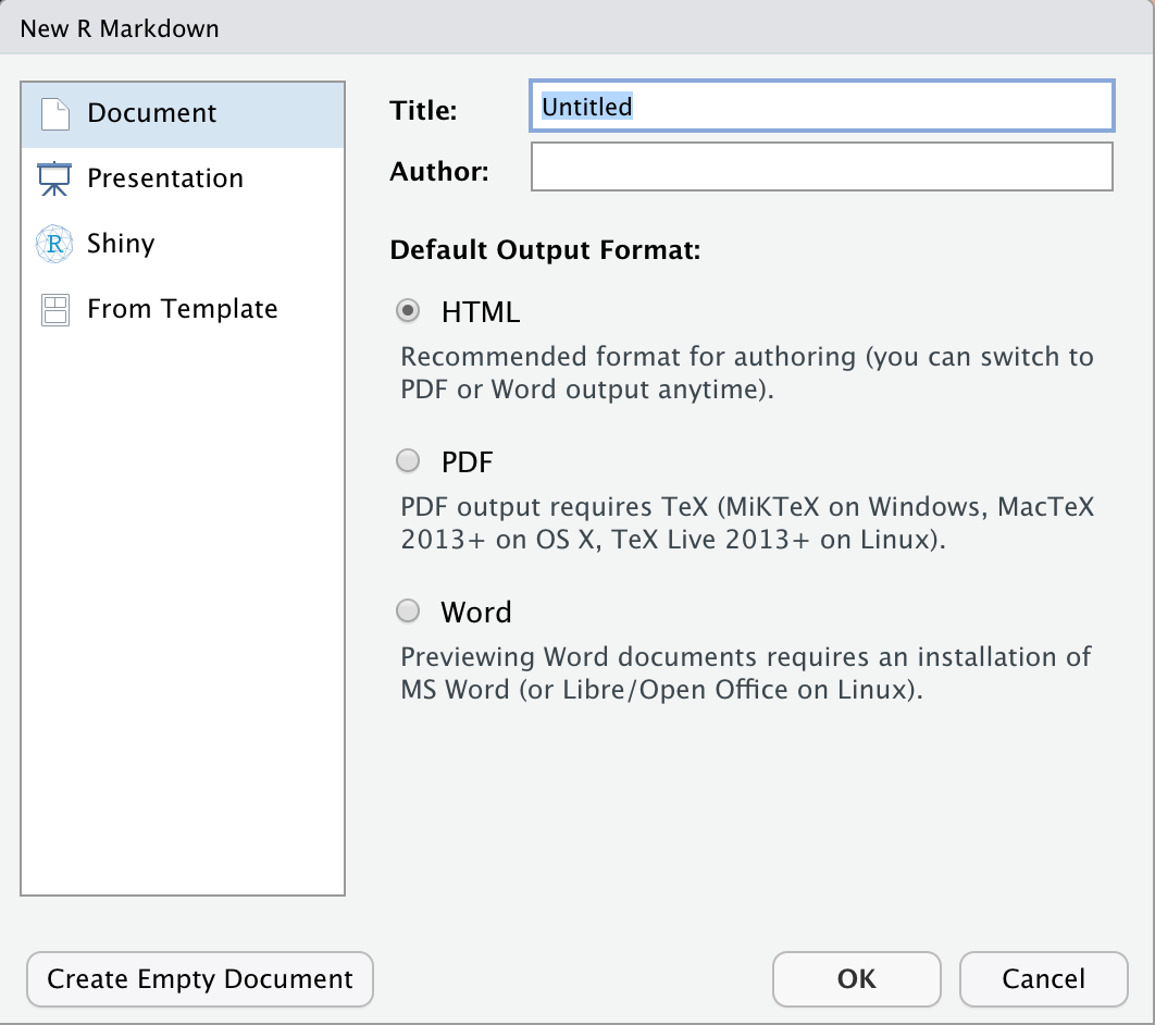
Figure 3: New R Markdown file

Use the default settings for HTML (we can always change it later), and click OK.

Once the Rmarkdown document appears and opens in RStudio, we should see something like this:

Figure 4: The blank R Markdown template

If you look at the top right of the code editor window, there’s a small “A” shaped compass¹.

If you click on that icon, the R Markdown document will render into something that is visually more appealing and essentially will look much more like a word processor might.

Figure 5: Visual markdown editor

You can toggle the outline/table of contents on and off with the button immediately to the left of the “A” shaped compass.

yaml header

yaml stands for yet another markup language. Save that for a trivia question in the future. Every Rmarkdown document uses a yaml header (the bits between the --- marks) at the top of the document to tell your computer how R should knit your document together (stitch all the different parts together into a single seamless document).

There are many possible options here and they can depend on the type of document we want to create, but typically the key pieces are:

• title: Name of our document
• output: what we end up knitting our R markdown into (e.g., .pdf, .html, .docx). See the RStudio R Markdown website for more details on different format options.

Note, spacing and indentation matters in yaml. If we’d like to specify additional options for a specific output, we need to add more lines and indent the argument we want to add.

Let’s focus on making an .html file, and add some parameters about the table of contents. We can add toc: true and toc_float: true to our yaml so it looks like this:

---
title: "Untitled"
output: 
  html_document:
    toc: true
    toc_float: true
---

Now each section and subsection of our document will appear in the table of contents. How do we make a section or subsection? Read on!

Body Text

The body of our document is typically text written in Markdown². Markdown is a simple text language that helps make it very easy to just sit down and type without worrying about formatting, and it works across many different operating systems and applications. There are a few basic formatting options to do things like make font bold, italicized, add numbered or bulleted lists, or add section headers. To learn more, while in RStudio, go to the menu and locate Help at the top of the screen. Under Help > Markdown Quick Reference you’ll find a handy “cheatsheet” to help learn these options. There are many additional RStudio cheatsheets for many topics here, and a specific pdf on using R Markdown is available as a pdf here.

For example, to add a figure using Markdown, we can use the following:

![alternate text](happy_face.png)

We’ll talk more about how to customize image sizes and add captions within RMarkdown later in this module.

Illustration by @allison_horst

code chunks

The third and final component of an R Markdown document is what makes it R Markdown. The inclusion of code! What’s great is while the default is typically R code, there are quite a few additional code language options that can be stitched together. Look for the little +C icon in green at the top of your R Markdown, or go to Code > Insert Chunk. The keyboard shortcut to do this is Ctrl + Alt + i.

Let’s go ahead and create a new R code chunk and look at some of the chunk options.

```{r}
# my empty code chunk!
```

There are many code chunk options we can use. Put your cursor after the {r, and hit tab. There are tons! If you want to learn more, check the R Markdown reference guide. The key options that we want to know:

• echo: TRUE or FALSE. If TRUE, whatever code we put in the chunk will be displayed when we knit the document.
• eval: TRUE or FALSE. If TRUE, the code inside the chunk will be evaluated or run.
• include: TRUE or FALSE. If FALSE, the code is still run, but the results won’t be displayed and neither will the code.³
• fig.cap: A quoted character string, adds captions to figures from code outputs. One caption per chunk.
• out.width/out.height: A quoted percentage, i.e., “100%”. This controls the size of the image being output from a given code chunk. Very easy and effective for changing graphic output sizes.

Knit Early and Often

One thing that makes writing in R Markdown fun is the ability to get instant feedback. Clicking the Knit button when a section of your document has been updated will (re)-generate the document. We can change the default location the outputs appear by changing the options via the little gear wheel to the right of the knit button. Look for “Preview in Viewer Pane” and select it. From that point on, every time you click knit, most outputs should appear in the Viewer pane of RStudio.

Knitting frequently can be tedious if you have a large document with lots of figures or visuals. However, it’s a great way to learn, and also to ensure things are rendering correctly and successfully.

Customizing Visuals

There’s lots of great visualization materials out there, but there are a few helpful tips to keep in mind when using images or graphics in your R Markdown documents. While the default Markdown option does permit adding images with the ![](image.png) syntax, it doesn’t permit as much fine control.

If we use a handy function from the {knitr} package, we can have more more concise control over the size and placement of an image without having to learn a lot of special code. For example, we can use either a local file path, or a url! In addition we can add some arguments that help us specify the size of the image, using the out.width or out.height parameters. Finally, we can add a caption with fig.cap. Note, here we want to hide the code and just show the image, so we use echo=FALSE.

By using fig.cap in the code chunk, the figure caption numbers will be automagically assigned and updated each time you knit

```{r rivphoto, echo=FALSE, out.width='80%', fig.cap="A tranquil river (photo: R Peek)"}

knitr::include_graphics("images/river_peek.JPG")

```

Figure 6: A tranquil river (photo: R Peek)

Similarly, we can include a URL.

```{r delta, echo=FALSE, fig.cap="Sacramento-San Joaquin Delta, color infrared (image: R Pauloo)"}

url <- "https://raw.githubusercontent.com/richpauloo/rp/master/static/img/delta_cir_2.png"
knitr::include_graphics(url)

```

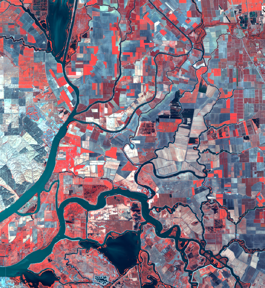
Figure 7: Sacramento-San Joaquin Delta, color infrared (image: R Pauloo)

Tables

Sharing data in tables is a common need for reporting, summary, and analysis. There are a number of packages in R that may be helpful for making tables. This list is not exhaustive, and is meant to just show a few options that may be useful.

• {DT}: Great for interactive and dynamic html based tables
• {kable} & {kableExtra}: Highly customizable static or dynamic tables
• {gt}: Very customizable static or dynamic tables

Let’s load some data we can play with. We’ll use some existing datasets that come with packages you already have installed. The {dplyr} package comes with a number of different datasets, as do many R packages⁴. We’ll use the storms dataset since it’s large (+10,000 observations), and our nwis_sites from the American River which we created in a previous module.

# large dataset: dplyr::storms
storms <- dplyr::storms

# sites
nwis_sites <- read_csv("data/nwis_sites_american_river.csv")

For large unwieldy tables that you may want to just be able to quickly search or explore, the {DT} package is great, especially for .html documents. Let’s make a table of the storms data. A nice feature of the datatable() is we can search and filter our table interactively.

library(DT)

storms %>% 
  slice(1:200) %>% # take first 100 rows
  datatable() # that's it!

For a quick and easy static table, the kable() function from {knitr} is great. We can simply pass a dataframe to the function and we get a table! For more fancy options, we can use the functions from the {kableExtra} package.

library(knitr)
storms %>% 
  slice(1:10) %>% # take first 10 rows
  kable()

name	year	month	day	hour	lat	long	status	category	wind	pressure	tropicalstorm_force_diameter	hurricane_force_diameter
Amy	1975	6	27	0	27.5	-79.0	tropical depression	-1	25	1013	NA	NA
Amy	1975	6	27	6	28.5	-79.0	tropical depression	-1	25	1013	NA	NA
Amy	1975	6	27	12	29.5	-79.0	tropical depression	-1	25	1013	NA	NA
Amy	1975	6	27	18	30.5	-79.0	tropical depression	-1	25	1013	NA	NA
Amy	1975	6	28	0	31.5	-78.8	tropical depression	-1	25	1012	NA	NA
Amy	1975	6	28	6	32.4	-78.7	tropical depression	-1	25	1012	NA	NA
Amy	1975	6	28	12	33.3	-78.0	tropical depression	-1	25	1011	NA	NA
Amy	1975	6	28	18	34.0	-77.0	tropical depression	-1	30	1006	NA	NA
Amy	1975	6	29	0	34.4	-75.8	tropical storm	0	35	1004	NA	NA
Amy	1975	6	29	6	34.0	-74.8	tropical storm	0	40	1002	NA	NA

Here’s a slightly fancier option using {kableExtra}. See the great vignette for more details.

library(kableExtra)

storms %>% 
  slice(1:10) %>% # take first 10 rows
  kbl() %>%
  kable_paper("hover", full_width = T)

name	year	month	day	hour	lat	long	status	category	wind	pressure	tropicalstorm_force_diameter	hurricane_force_diameter
Amy	1975	6	27	0	27.5	-79.0	tropical depression	-1	25	1013	NA	NA
Amy	1975	6	27	6	28.5	-79.0	tropical depression	-1	25	1013	NA	NA
Amy	1975	6	27	12	29.5	-79.0	tropical depression	-1	25	1013	NA	NA
Amy	1975	6	27	18	30.5	-79.0	tropical depression	-1	25	1013	NA	NA
Amy	1975	6	28	0	31.5	-78.8	tropical depression	-1	25	1012	NA	NA
Amy	1975	6	28	6	32.4	-78.7	tropical depression	-1	25	1012	NA	NA
Amy	1975	6	28	12	33.3	-78.0	tropical depression	-1	25	1011	NA	NA
Amy	1975	6	28	18	34.0	-77.0	tropical depression	-1	30	1006	NA	NA
Amy	1975	6	29	0	34.4	-75.8	tropical storm	0	35	1004	NA	NA
Amy	1975	6	29	6	34.0	-74.8	tropical storm	0	40	1002	NA	NA

For nicely formatted tables and lots of control, the {gt} package is good. It does take a little more wrangling to get things formatted, but there’s great documentation for this package as well.

library(gt)
tab1 <- nwis_sites %>% 
  select(-sourceName) %>% 
  slice(1:10) %>% # get just first 10 rows 
  gt()

tab2 <- tab1 %>%
  cols_label(identifier = "NWIS ID",
             comid = "COMID",
             X = "Longitude",
             Y = "Latitude") %>% 
  tab_header(
    title = "NWIS Sites on the American River",
    subtitle = "Downstream of Nimbus, Sacramento County") %>% 
  fmt_number(
    columns = vars(identifier, comid),
    decimals = 0, use_seps = FALSE)
tab2

NWIS Sites on the American River
Downstream of Nimbus, Sacramento County
NWIS ID	COMID	Longitude	Latitude
11446500	948021150	-121.2277	38.63546
383729121181000	15025011	-121.3038	38.62463
11447540	15039173	-121.5206	38.56832
383438121204200	15024993	-121.3461	38.57713
383609121293200	15024919	-121.4933	38.60240
383052121324401	15039157	-121.5456	38.51454
383205121310901	15039157	-121.5192	38.53481
383457121254900	15024941	-121.4313	38.58241
383515121264400	15024941	-121.4466	38.58741
11446980	15024969	-121.3883	38.56713

Interactive Maps

And as you’ve seen from previous modules, we can also add maps! This is also a really nice way to share lots of information. We can only add {mapview} maps if we are using an html-based output, but they work well in R Markdown.

Let’s plot our NWIS Stations from the American River that we already loaded above. First we need to convert these data to {sf}. Let’s show code that does that. Remember to use eval=TRUE and echo=TRUE! One additional tip is to label your R code chunks. This helps us troubleshoot when things are not knitting properly, and helps keep things organized.

Code chunk labels show up in the outline, so making them informative is good. Note that we can only use characters and “-” in a code chunk label!

```{r make-nwis-sf, echo=TRUE, eval=TRUE}

library(sf)
# make nwis_sites spatial by converting to sf
nwis_sites_sf <- st_as_sf(nwis_sites, coords=c("X", "Y"), remove=FALSE, crs=4326)

```

Next we can make our map with mapview(). Note, there may be a minor rendering issue with {mapview}. Adding fgb=FALSE seems to address this!⁵ Note, here we are going to hide our code (echo = FALSE in the code chunk options) so that we only show the results!

Extending R Markdown

We’ve demonstrated that R Markdown can be used for creating html files. This is the tip of the iceberg, and the foundation of building websites and dashboards with Rmd. Remember that Rmd files can also knit to .doc and .pdf files, although we don’t cover it in this module. Also, because Rmd files are code, as you level up your R skills, you can begin to automate generating tens, hundreds, even thousands of reports from a single template. To extend your understanding of the capabilities of Rmd, check out One R Markdown document, 14 demos, a video of a talk by R Markdown creator and developer Yihui Xie at rstudio::conf(2020).

Additional Resources

There many different types of outputs possible, including slide presentations (see {xaringan} and RStudio’s page on slides), pdfs, and word docs.

Here’s a sample of some good resources that are freely available online:

• One R Markdown document, 14 demos: a video of a talk by R Markdown creator and developer Yihui Xie at rstudio::conf(2020)
  
• R Markdown (online book): all the tips and details you could ever want
• Tips for Working with Images in R Markdown: Helpful tips on sizing and image resolution
• Working with pdf’s via R Markdown using the {tinytex} package: you’ll need a LaTeX distribution installed in order to render or knit to pdf. The {tinytex} package is a great solution.

Previous module:
12. EDA Next module:
14. Troubleshooting

---

1. Drafting compasses are really cool.↩︎

2. Read more on the simple markup language Markdown here.↩︎

3. Code that has been evaluated in one chunk can be referred to or used in subsequent chunks. So you can load objects at the start of your document and use them throughout the entire document.↩︎

4. To figure out what datasets are available across all installed packages, try data(package = .packages(all.available = TRUE)).↩︎

5. {mapview} is not a static package. Rather, it’s under active development. At the time of writing, the solution to inserting mapview objects into an html document is to use mapviewOptions(fgb=FALSE). In the future, this may change so that it’s not needed and mapview objects in an html document “just work”. A benefit of using open source projects is that conversations about these fixes and updates can sometimes come from the package developers themselves, as in the case of this mapview issue discussed on Github that provided our fix.

   ```{r make-nwis-mapview, echo=FALSE, eval=TRUE}

   library(mapview) mapviewOptions(fgb=FALSE)

   mapview(nwis_sites_sf, col.regions=“cyan4”, layer=“NWIS Sites”)

   ```↩︎