4. Interactive Visualization

Having fun with interactivity in R

Learning objectives

• How to use interactive visualization in R
• Workflows to go from data to visualization
• Understand a visualization objective

Why interactive visualizations?

One of the most exciting and rewarding parts of learning to code is the ability to see results! Visualization is one of R’s strengths, and there are a seemingly constantly growing number of packages that can assist you in customizing just about any visualization you can think of. Importantly, this allows users to access and interact with data on a level that would not otherwise be possible.

Because we can learn new things and develop new questions by effectively interacting with data, the ability to stitch raw data into something visual can help provide unique insight that may be much harder to discern with a table or some raw data.

Let’s demonstrate a simple way we can collect data, update it automagically, and visualize in a fairly streamlined manner. Keep in mind, this is one approach, but there are many more, with increasing complexity. But for illustration, “working” examples (as in, it works when you try it!) are the best way to build your proficiency in R programming.

Mapping with Geocoder

This example will couple the power of collecting user input (favorite places to eat/drink) with interactive mapping. We’ll use a Form to collect some data, and then display that via a map. This illustrates some of the power (and fun!) of programming in R.

Collect Data

Answer as many questions as you feel comfortable, but at minimum, the street address/name of your favorite place to eat or get a beverage (hot or cold).

Import and Map Data

We’ll need these packages to work with this data.

library(tidygeocoder) # geocode our addresses
library(tidyverse)    # wrangle data
library(janitor)      # clean column names
library(glue)         # modern paste() function
library(sf)           # make spatial data
library(mapview)      # interactive maps!
mapviewOptions(fgb = FALSE)

The entire script we need is below (don’t forget to include the packages above). To generate a public .csv from a Form, we can use File > Publish to the Web¹. Importantly, here we are publishing to a .csv so we can read the data in directly and simply using read_csv. We then clean, convert it into an sf object, and map!

# the url for the Form data 
form_data <- paste0("https://docs.google.com/spreadsheets/d/e/",
                    "2PACX-1vSODxBm_z5Gu8a42C6ZFEa3S5iTbYV-",
                    "qucCGvasGS6c0qFUAml5vSMEgbvI9PYo1HJ20Y_WY62aTAb-",
                    "/pub?gid=1462593645&single=true&output=csv")

# read in url and clean
dat <- read_csv(form_data) %>% 
  clean_names() %>% 
  rename( dining_name = 3, dining_address = 4)

# geocode using Open Street Map (osm) API because it's free
dat_geo <- dat %>%
  geocode(dining_address, method = 'osm', lat = latitude , long = longitude)

# make into sf object so we can map
dat_geo <- dat_geo %>% 
  filter(!is.na(latitude) & !is.na(longitude)) %>% 
  st_as_sf(coords = c("longitude", "latitude"), crs = 4326, remove = FALSE)

# map!
mapview(
  dat_geo, 
  zcol = "comfort_using_r", 
  layer.name = "R comfort level", 
  cex = 6.5
)

Use {leaflet}

We used {mapview} above, but we could also use the {leaflet} package to make a more customizable map with some fancy icons and a measuring tool, to calculate how far each location is from a point of interest, or the the total area that encompasses all our points.

library(leafpm)
library(leaflet)
library(leaflet.extras)
library(htmltools)

# set up our map
m <- leaflet() %>%
  # add tiles or the "basemaps"
  addTiles(group = "OSM") %>% # defaults to Open Street Maps
  addProviderTiles(providers$CartoDB.Positron, group = "Positron") %>% 
  addProviderTiles(providers$Stamen.TonerLite, group = "Toner Lite") %>%
  addCircleMarkers(
    lng = -121.4944, lat = 38.5816, fillColor = "red", color = "black",
    popup = "Sacramento!", group = "Home",
  ) %>% 
  addCircleMarkers(
    data = dat_geo, group = "Food & Drink",
    label = ~htmlEscape(first_name),
    popup = glue(
      "<b>Name:</b> {dat_geo$first_name}<br>
      <b>Food_Name:</b> {dat_geo$dining_name}<br>
      <b>Food_Address:</b> {dat_geo$dining_address}<br>
      <b>R comfort (1-10):</b> {dat_geo$comfort_using_r}"
    )
  )  %>% 
  addLayersControl(
    baseGroups = c("Toner Lite", "Positron", "OSM"),
    overlayGroups = c("Home", "Food & Drink"),
    options = layersControlOptions(collapsed = FALSE)
  ) %>% 
  addMeasure()

m  # Print the map

Using D3

A powerful visualization tool is the D3.js (javascript) library, which has some amazing options. What’s great is there are ways to easily translate your R code into D3, via packages like {r2d3}.

Here’s an example of a calendar visualization, based on the stock market open and close between 2006 and 2010.

A Network with D3

Another example of a way to interactively engage with data is networks. Here’s a simple example of an interactive network visualization:

# Libraries
library(igraph)
library(networkD3)

# create a dataset:
data <- tibble(
  from = c(
    "Dam","Dam","Dam", "Dam",
    "River","River","River", "River","River",
    "Canal", "Canal", 
    "Diversion","Diversion", 
    "Reservoir", "Reservoir","Reservoir",
    "Lake","Lake","Lake", "Lake", 
    "Road","Road","Road",
    "Culvert", "Culvert",
    "Fish", "Fish","Fish",
    "Frog","Frog","Frog",
    "MacroInvertebrates","MacroInvertebrates"
  ),
  to = c(
    "River","Reservoir","Canal","Diversion",
    "Lake","Reservoir","Frog","Fish","MacroInvertebrates",
    "Diversion", "Reservoir",
    "Dam", "River",
    "River","Dam","Fish",
    "Fish","Dam","Frog","MacroInvertebrates",
    "Fish","Dam", "Canal",
    "Road", "Dam",
    "Frog", "River","MacroInvertebrates",
    "Fish", "River", "Lake",
    "River", "Lake"
  )
)

# Plot
(p <- simpleNetwork(data, height = "600px", width = "600px", 
                    fontSize = 16, fontFamily = "serif",
                    nodeColour = "darkblue", linkColour = "steelblue",
                    opacity = 0.9, zoom = FALSE, charge = -500))

When we wrap code with (), as we did with the plot above, it will evaluate the code and provide the output in the Console, Plots, or Viewer tab (depending on the code). This is a handy shortcut instead of having to save the object p <- my_code and then call/print the object p. We use (p <- my_code).

If we wanted to save this interactive visualization and send it as a standalone .html file, we could use the following code:

# save the widget
library(htmlwidgets)
saveWidget(p, file = "output/network_interactive.html")

Plotly

Another great tool for interacting with data is the {plotly} package, which if using the {ggplot2} framework, has a very handy ggplotly() function which you can wrap around pretty much any ggplot to turn a static plot into an interactive one. This allows you to click, hover, zoom, etc. inside your plot, and is a very useful tool for exploring data.

For example, say you were asked to find the date of a peak flow for a given year, or an outlier in a graph. We could figure this out with dplyr::filter() and additional queries of our data, but it would also be easy to visually look and see the date of peak flow on a plot. This is where the power of plotly can be very helpful.

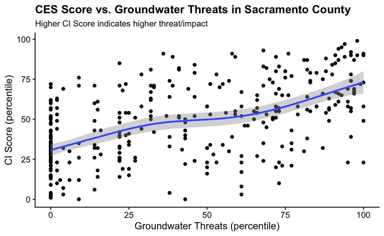
Let’s use the CalEnviroScreen data from Sacramento County from a previous module. Recall, higher scores mean a higher impact of pollution to a community.

# load CES data for Sacramento county
ces3_sac <- readRDS("data/ces3_sac.rds")

mapview(ces3_sac, zcol = "CIscoreP")